To be more general here in the introduction, the situation is that we have a user-item preference matrix which is also evolving over time. Essentially, we have a collection of user-item preference matrices, one for each time point. The preference matrix can be, for example, user’s preference on a collection of books, popularity of movies among people, effectiveness of a set keywords on a collection of campaigns. The prediction task is really to forecast a user-item preference matrix of the next time point.
From another angle, we really have a 3D preference matrix of with axes being users, items, and time. Given the matrix, the task is to predict a future slice of the matrix along the time axis.
The problem is very interesting and makes a lot sense in the real world. For example, the cinema can predict which movies will be popular next day/week/month, and make arrangements according to the predictions to maximize the profit.
Table of content
Link to the code
- permanent link to code https://github.com/hongyusu/SparkViaPython/tree/master/Examples/Campanja_codes/.
- Code for Custom B is only slightly different from code for custom A.
Coding
I would use Python for coding on top of Spark environment. Some Python packages involved and worth of mentioning are listed as follows.
numpyfor array and matrix operation.pandasfor data preprocessing and transformationsklearnfor machine learning model, e.g., random forest regression running on a single cpu core.mllib, Spark machine learning library for machine learning models e.g., collaborative filtering running parallel on Spark environment.matplotlibfor plotting.pysparkSpark python context enabling python on Spark.statsmodelsfor autoregressive-moving-average ARMAR model on time series prediction.
The reasons are
- It is essentially log data generated possibly from some streaming system e.g., Kafka.
- The example data file is small compared to the real situation. The preprocessing and learning should be able to scale on very large dataset. Therefore, the given task naturally requires framework like Spark or Hadoop.
- During the data preprocessing and exploration, a lot of operations are done based on key/value pairs.
MapReduceheuristics will naturally optimize these key/value operations. - Machine learning is also expected to be scalable on large scale data. Spark has a machine learning library with parallelized learning algorithms.
Complete code for customer A and results are in my Github.
Complete code for customer B and results are in my Github.
Code can be run in Spark with the following command (in my case)
$../../spark-1.4.1-bin-hadoop2.6/bin/spark-submit solution.pyQuestion 1: Modeling
I would use collaborative filtering to impute missing values then random forest regression trained locally for each individual keyword.
Data exploration
Overview
-
There are 93 days. Logs are available for each day.
First day Last day Actual date 2015-08-17 2015-11-17 Index 0 92 -
About 1.19% criterions are not unique to ad group meaning that keyword can be defined as
adgroup_id+criterion_id. On the hand, 57.04% keywords are not unique to campaign meaning that I cannot combinekeyword_idandcampaign_id. Different campaigns share keywords. -
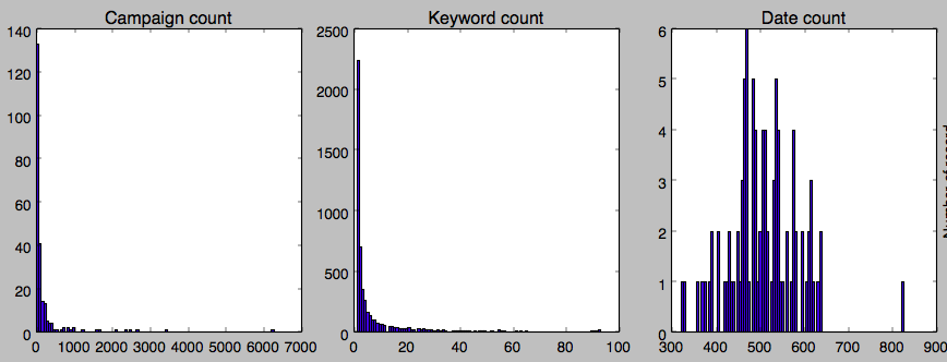
The histogram of the number of logs for campaign, keyword and date are shown in the following figure.
-
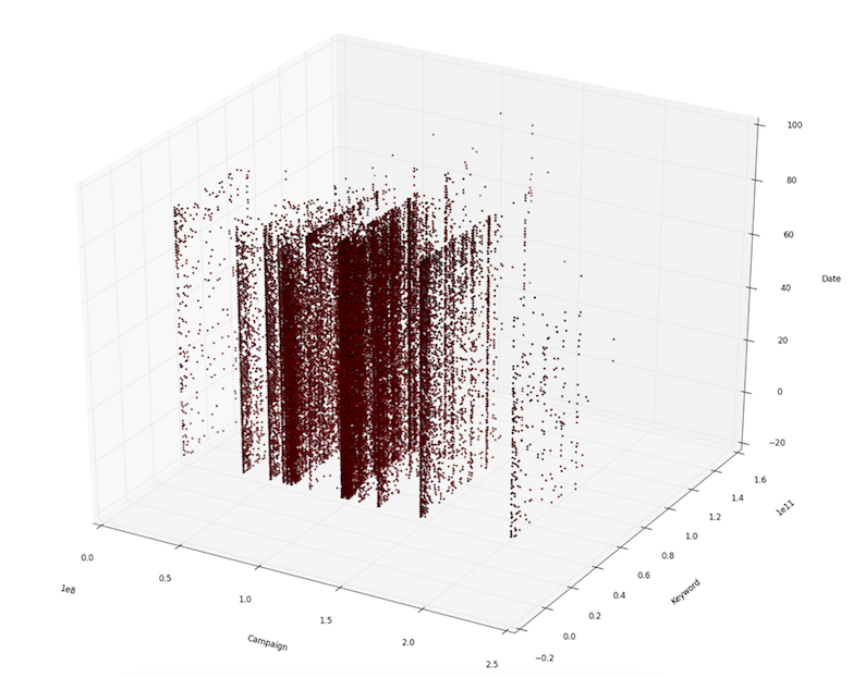
The availability of logs in campaign/keyword/date is shown in the following figure. The figure demonstrates
- The date can be seen as a preference matrix of keywords on campaigns over time (time series preference matrices).
- Different campaigns share keywords.
- Data are very sparse.
-
Ideally, I would model the data with all dimensions (campaign, keyword, time). However, due to the sparseness, I will collapse the campaign-keyword-time matrix to a keyword-time matrix by summing along the campaign dimension.
-
In particular, I will work with the keyword-time matrix in the following part of the analysis.
Behavior of an average keyword over time
-
The following plot shows the global behavior (mean keyword) over time, shown separately for different
match_typeand the number ofclickfor individual log.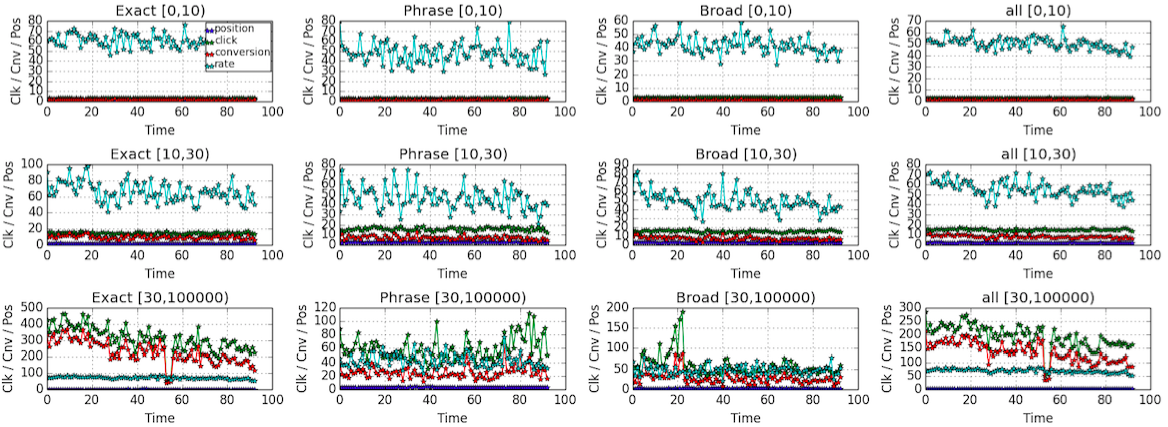
-
There is a
heart beat/periodical pattern in the plot above. However, the different between differentmatch_typeis quite small. Again, I would ideally model the data with differentmatch_type. However, I would average overmatch_typedue to the sparseness. -
The following plot shows the global behavior over time, without making difference on
match_type.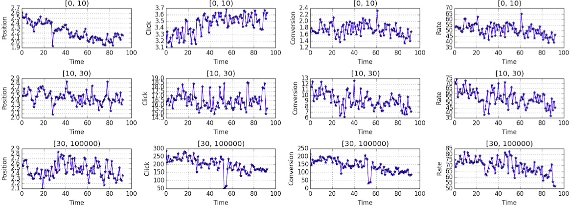
Behavior of individual keyword over time
-
Looking at the behavior of individual keyword, I also observe the periodical pattern of having high
clicktypically on Monday and Sunday and lowclickduring the working days. However, the patterns are quite different from one keyword to another as shown in the following plot.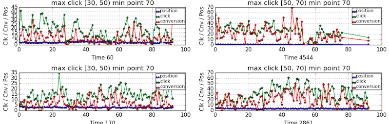
-
If there is a pattern base on weekdays, how about average over weekdays? The following plot shows the behavior of individual keyword averaged over weekdays. The pattern is somehow more clear that people did more searches at the beginning or towards the end of the week while did fewer searches during the week.
-
The observations suggest that it might be a good idea to build a regression model based on weekdays. For example, use data from previous Monday to Sunday to predict current Monday, and use data from previous Tuesday to this Monday to predict this Tuesday.
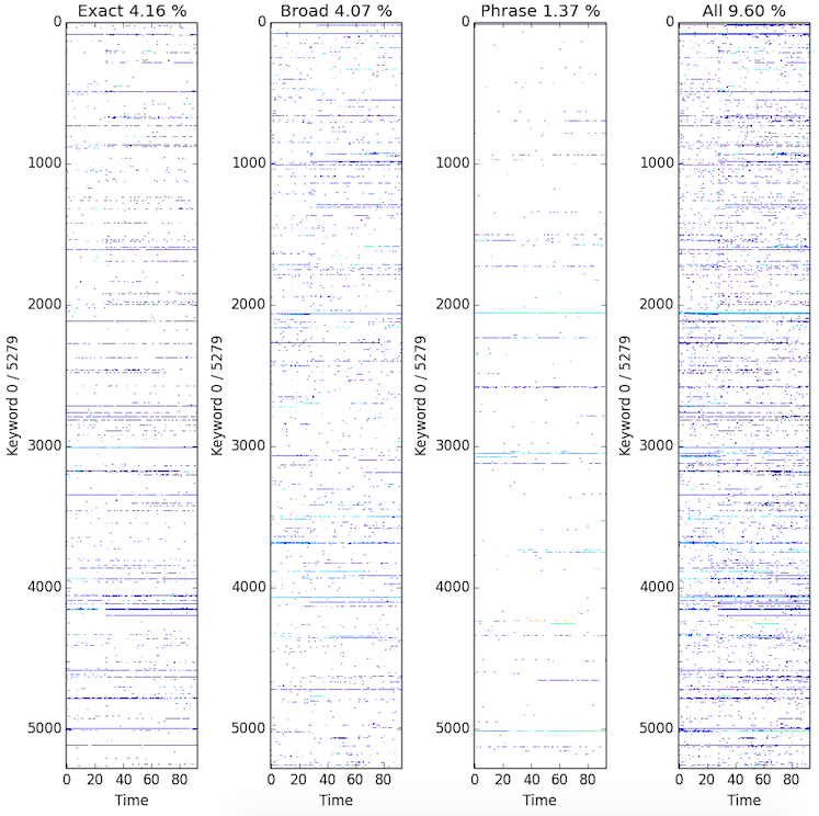
Missing data
For now the practical problem is really how much data I actually have or can use. The following plots show all available data points in keyword-time matrix in terms of different match type. The plot demonstrates that
-
Different matching type generates different entries in the data matrix since the individual percentages sum up to the
all. -
Interesting! This actually says that different
match typedid not generate overlapped data. -
In addition, I only have about 10% data available in the matrix by putting together data generated from different
match type. -
It actually suggests that to deal with sparseness I should really pool data together other than model them in high resolution.
Learning and prediction
So far, the hints from basic analysis are
- I should pool
keyworddata from different campaigns and match types to tackle the sparseness. - The data is still very sparse even pooling logs from different dimensions. We still need to work out the missing values in the matrix.
- There is a
heart beat/weekdaypattern for different keywords across time which essentially goes up at the beginning or towards the end of the week and goes down during the week. The periodical pattern suggests that the preference of different keywords are somehow correlated because of the human behaviour. In machine learning, it allowscollaborativeanalysis e.g., collaborative filtering. - Another patten shown in the data besides periodical pattern is that the number of clicks/conversions decay over weeks.
- Behavior of individual keywords are quite different which means that local regression model built based on individual keyword might be a good idea. However, with additional/external data, one can group keywords into different keyword groups and build a regression model for each group.
- I should focus on predicting
clickandconversiondata, as the ratio is the conversion rate.
Missing value imputation
-
As already mentioned, the first problem is that I need to compute the missing values in the keyword-time matrix of click data and conversion data.
-
This can be tackled by collaborative filtering. The technique is well-known for recommender system and is implemented in Spark machine learning library. The actual algorithm running in the backend is alternating least square ALS.
-
In particular, I will be working on a keyword-time matrix
Item Value Missing entry 443835 All entry 490947 Missing at 90.40 % Keywords 5279 Time 93 -
For now, I only divide all data into training and test where test data is just to make prediction on the last day. Parameter tuning is done on training data. Then model is trained with the best parameters.
-
Parameter selection result is listed as in the following table.
Rank Lambda NumIter RMSE 30 0.100 10 1.64 30 0.100 15 1.62 30 0.100 20 1.60 30 0.010 10 1.50 30 0.010 15 1.45 30 0.010 20 1.42 30 0.001 10 1.50 30 0.001 15 1.44 30 0.001 20 1.44 20 0.100 10 2.27 20 0.100 15 2.24 20 0.100 20 2.22 20 0.010 10 2.16 20 0.010 15 2.13 20 0.010 20 2.14 20 0.001 10 2.20 20 0.001 15 2.10 20 0.001 20 2.14 10 0.100 10 3.40 10 0.100 15 3.44 10 0.100 20 3.45 10 0.010 10 3.37 10 0.010 15 3.36 10 0.010 20 3.33 10 0.001 10 3.43 10 0.001 15 3.30 10 0.001 20 3.34 -
Compare collaborative filtering approach with mean imputation approach on
clickdata.Method RMSE CF 1.42 Mean imputation 93.47 -
The following figure shows the results of imputation on
clickdata for 4 keywords. Each subplot shows theclicknumber of thekeywordalong time. Vertical lines correspond to non-missing data.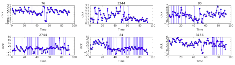
-
Similarly, parameter selection on
conversiondata is shown in the following table.Rank Lambda NumIter RMSE 30 0.100 10 1.63 30 0.100 15 1.62 30 0.100 20 1.60 30 0.010 10 1.50 30 0.010 15 1.45 30 0.010 20 1.43 30 0.001 10 1.51 30 0.001 15 1.45 30 0.001 20 1.42 20 0.100 10 2.27 20 0.100 15 2.22 20 0.100 20 2.22 20 0.010 10 2.15 20 0.010 15 2.13 20 0.010 20 2.13 20 0.001 10 2.17 20 0.001 15 2.13 20 0.001 20 2.13 10 0.100 10 3.55 10 0.100 15 3.41 10 0.100 20 3.42 10 0.010 10 3.35 10 0.010 15 3.30 10 0.010 20 3.29 10 0.001 10 3.37 10 0.001 15 3.34 10 0.001 20 3.29 -
Compare collaborative filtering approach with mean imputation approach on
conversiondata.Method RMSE CF 1.42 Mean imputation 93.47 -
The following figure shows the results of imputation on
conversiondata of 4 keywords. Each subplot shows theconversionnumber ofkeywordalong time. Vertical lines correspond to non-missing data.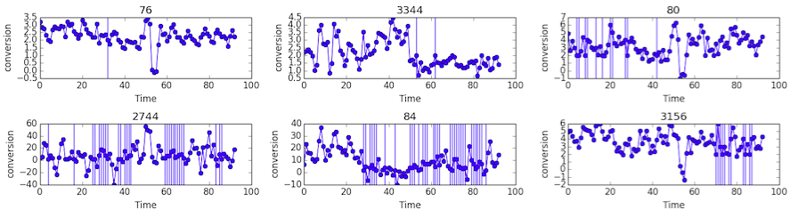
Localized regression model
-
The idea is to build a regression model locally for each keyword in order to capture the weekday pattern of clicks and conversions.
-
At the same time, the weekday regression model will not collapse for some keywords in which clicks/conversion decays over weeks.
-
In particular, I have for each keyword data from day 0 to day 92. The the final task is predict the value for day 93.
-
As training data x and y, I construct from historical data
X(Feature) Y(Label) day 0, day 1, …, day 6 7 day 1, day 2, …, day 7 8 … … day 85, day 86, …, day 91 92 day 86, day 87, …, day 92 ? -
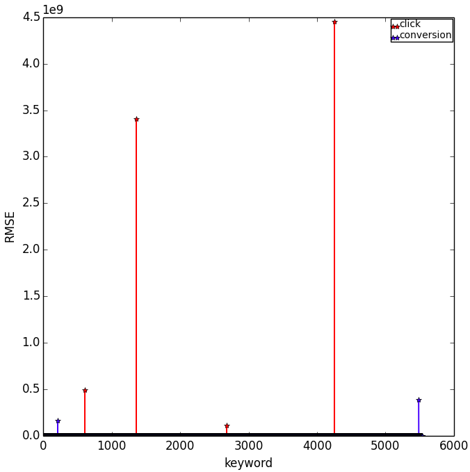
We use random forest regression model from
scikit-learn. The training rooted mean square error RMSE are shown in the following plot.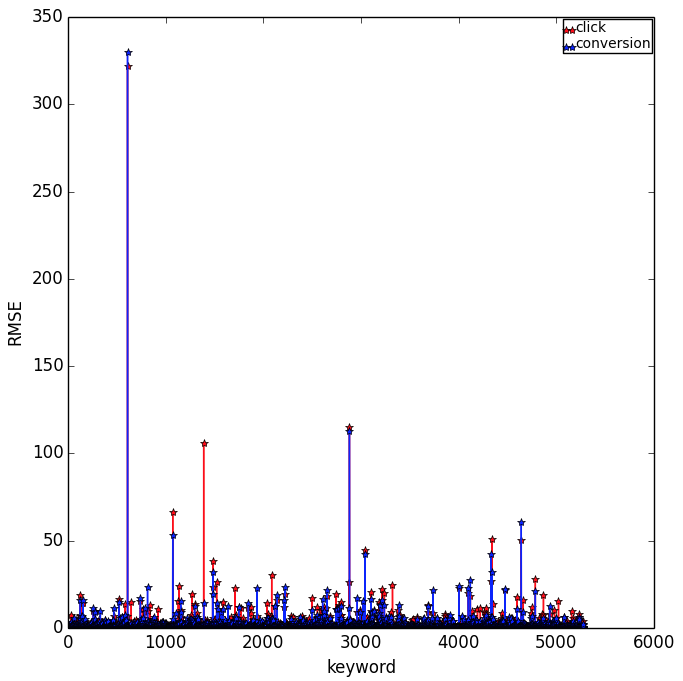
Other possibilities
-
The approach described here is collaborative filtering for missing value imputation + local regression model based on weekday pattern for individual keyword.
- Some improvement on current implementation:
- Log transformation of the
clickandconversiondata to make them more like Gaussian distributed. So that regression can be better trained. - Add parameter selection procedure on training local random forest regression model.
- Make training/validation/test partitions for parameter selection scheme.
- Log transformation of the
- Some improvement on current implementation:
-
Other possibilities base on current data
-
Missing value imputation + global regression for all keyword. The only difference here is to train a global regression model with all keyword data instead of having one regression model for individual keyword.
- Pro: Consider more information when making a prediction. More flexible for distributed computation.
- Con: Not sure whether other keywords are actually related to the current one.
-
Missing value imputation + group regression. Divide keywords into groups according to campaign information, then build a regression model for each keyword group.
- Pro: Consider other keyword in the same group. Model is trained with more information.
- Con: Sparse data which is difficult to find the keyword group.
-
Missing value imputation + time series prediction model e.g., autoregression model, autoregressive–moving-average model. Previous regression models are built based on the observation that there is a weekday pattern on the number of
clickorconversions. However, data here is essentially time series of the preference over keywords. Therefore, the time series regression can be applied here.- Pro: Data is essentially time series.
- Con: Local model on individual keyword. Neglect weekday pattern.
-
Gaussian process locally for each keyword. The observation for each keyword can be taken as a collection (21) of time series curves from Monday to Sunday. Gaussian process essentially assume observations on different day (e.g., Monday) follows a Gaussian distribution and the correlation between different days (e.g., Monday and Tuesday) follows a covariance structure.
- Pro: Advanced model for time series modeling. Training is still feasible on the data of this size. Prediction comes with confidence interview (variance).
- Cons GP is for finding patterns not for making prediction which means that the variance of prediction might be very high. Neglect the fact that the popularity of keywords decay over weeks.
-
Ensemble models combining multiple local/global regression models.
-
-
Given more data, it is really to make regression model on fine-tuned groups
- When
click/conversioncan be segmented on devices, it makes sense to predictclick,conversion,conversion ratefor each device. - When more information about keywords is available, it is then realistic to put keywords into different groups and run regression/missing value imputation on different group.
- When
Question 2: Pitfall
The assumption in regression $$y=wx+b$$ is the output variable $$y$$ is Gaussian distributed if input features are Gaussians which is true in most of cases. Therefore, if the number of conversions is few or zero, when learning the regression model, the distribution of $$y$$ is skewed.
- When the number of conversions is few, it might make sense to have a log transformation of the number of conversions. As a results, the distribution of the number of conversion is more like Gaussian.
- When the number of conversion is zero and there are many of it, it might be a good idea to have a two stage model. In the first stage, having a binary classifier/outlier detector to predict if the conversion of a keyword is zero or non-zero. In the second stage, building a regression model to predict the actual conversions for keyword predicted to have conversions in the first stage.
Question 3: Measure the performance
In order to compare the performance of two models (model A and model B) in term of predicting conversion rate, one can work on
- Historical data
- by comparing rooted mean square error (RMSE) computed from all available test data points.
- Future data
- by comparing rooted mean square error (RMSE) computed from all available test data points.
- by performing an
A/B testin order to claim that updating keywords by deploying model A significantly (statistically) boots the conversion rate compared to deploying model B.
On historical data
RMSE as measure of success
Conversion rate ($$R_{j}$$) of a keyword $$j$$ is defined as the ratio between the number of conversions and the number of clicks during a fixed sample period as
$$ ConversionRate = \frac{Conversion}{Click} $$
The sample period can be 1 day or a few hours. Essentially, the number of clicks and the number of conversions during the period are collected and assigned to the sample point at the end of the sample period. The conversion rate for the period is computed accordingly and also assigned to the sample point. The measure of success is the rooted mean square error (RMSE) between the true conversion rate $$R$$ and the predicted conversion rate $$\hat{R}$$ defined as
$$RMSE = \sqrt{\sum_{j=1}^{M}\sum_{i=1}^{N}(R_{ij}-\hat{R}_{ij})^2}$$
assuming there are $$M$$ keywords and $$N$$ time points.
The test procedure can be described as follows.
-
Assume we have historical data of conversion rate of $$M$$ keywords on N time points (e.g., N days)
$${{R_{ij}}{i=1}^{N}}{j=1}^{M}$$
-
With model A we are able to predict the conversion rate of $$M$$ keywords on N time points
$${{\hat{R}^A_{ij}}{i=1}^{N}}{j=1}^{M}$$
-
With model B we are able to predict the conversion rate of $$M$$ keywords on N time points
$${{\hat{R}^B_{ij}}{i=1}^{N}}{j=1}^{M}$$
-
Rooted mean square error of two models are computed according to
$$RMSE_A = \sqrt{\sum_{i=1}^{N}\sum_{j=1}^{M}(R_{ij}-\hat{R}^A_{ij})^2}$$
$$RMSE_B = \sqrt{\sum_{i=1}^{N}\sum_{j=1}^{M}(R_{ij}-\hat{R}^B_{ij})^2}$$
-
We say model A outperforms model B in predicting conversion rate if RMSE of A is smaller than RMSE of B.
-
Pro:
- The test is fast and cheap.
-
Con:
- The problem is that the difference between two RMSEs might be very small or due to some randomness. Therefore, the claim based on RMSE might not be very well justified.
- Overfit training data if the test is not conducted in a proper way.
On future data
In stead of testing the model on historical data, one can perform the test on line. For example, if the sample period is 1 day, one can predict the conversion rate of tomorrow using all data available upto today; then repeat on the following days.
RMSE as measure of success
In stead of testing the model on historical data, one can perform the test in a online fashion. For example, if the sample period is 1 day, one can predict the conversion rate of tomorrow using all data available upto today; then repeat on the following days.
The test procedure is described as follows.
-
Assume we have some data available for training which allow us to predict (with model A and model B) the conversion rate of of $$M$$ keywords for tomorrow (day 1)
$${\hat{R}^B_{j1}}{j=1}^{M} , {\hat{R}^B{j1}}_{j=1}^{M}$$
-
The next day we will collect the real conversion rates for $$M$$ keywords
$${R^B_{j1}}_{j=1}^{M}$$
-
The procedure can be repeated for $$N$$ days in the future. In the end we will collect the true conversion rates of $$M$$ keywords
$${{R_{ij}}{i=1}^{N}}{j=1}^{M}$$
conversion rates of $$M$$ keywords predicted by model A
$${{\hat{R}^A_{ij}}{i=1}^{N}}{j=1}^{M}$$
conversion rates of $$M$$ keywords predicted by model B
$${{\hat{R}^B_{ij}}{i=1}^{N}}{j=1}^{M}$$
-
Rooted mean square error of two models are computed according to
$$RMSE_A = \sqrt{\sum_{i=1}^{N}\sum_{j=1}^{M}(R_{ij}-\hat{R}^A_{ij})^2}$$
$$RMSE_B = \sqrt{\sum_{i=1}^{N}\sum_{j=1}^{M}(R_{ij}-\hat{R}^B_{ij})^2}$$
-
We say model A outperforms model B in predicting conversion rate if RMSE of A is smaller than RMSE of B.
- Pro:
- Less likely to overfit training data compared to testing on historical data
- Con:
- The problem is that the difference between two RMSEs might be very small or due to some randomness. Therefore, the claim based on RMSE might not be very well justified.
- Take time and money to perform the test.
- Two models predict on a fix collection of keywords over time which does not make much sense and gain addition profits.
- Pro:
Conversion rate as measure of success (A/B test)
The model developed for predicting conversion rates of keywords is eventually applied to picking keywords during the campaign. Therefore, to compare model A and model B, it also make sense to measure the conversion rate over a collection of clicks from keywords suggested by model A and a collection clicks from keywords by model B over a certain time period.
The idea behind: if model A outperforms model B in predicting conversion rate of keywords, it will pick/update to a better collection of keywords and during the campaign period and such generate more conversions given a same amount of clicks.
-
The first problem is how many clicks are needed for the experiment. Assume the conversion rate in the group where model A is applied is $$p=60%$$. In order to say, with statistical power of $$\beta = 90%$$ and confident level of $$\alpha = 99%$$, that I can detect the conversion rate of q in group where model B is applied that is significantly different from p in A, I need $$M$$ clicks (samples). $$M$$ can be computed from
$$M = 2(t_{\frac{\alpha}{2}} + t_{\beta})^2\frac{p(1-p)}{|q-p|^2}$$
where $$t_{\frac{\alpha}{2}} = 2.58$$ and $$t_{\beta} = 1.29$$ are from the standard norm distribution table.
In particular, the sample size $$M$$ is shown in the following table when conversion rate from model A is $$60%$$
Conversion rate q in B is detected with statistical power Number of clicks 0.61 71889 0.62 17972 0.63 7988 0.64 4493 0.65 2876 -
The next thing is to collect click data. One has to make sure there is no bias towards special dates, people, products, regions, etc. For example, model A and model B will both work for similar campaigns from a same company on similar product in same regions over one week.
-
After sample collection, we have the number of clicks collected from group A and group B. We also know how many conversions are from each group. I would use standard G test to test wether conversion rate in A is different from conversion rate in B.
Custom B data
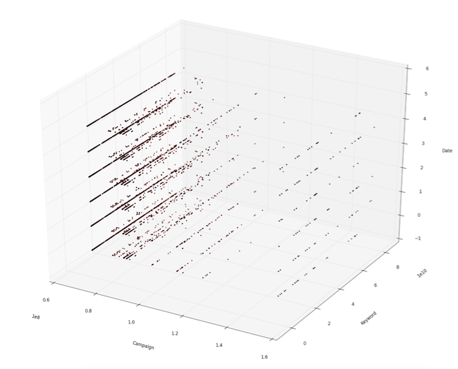
Overview
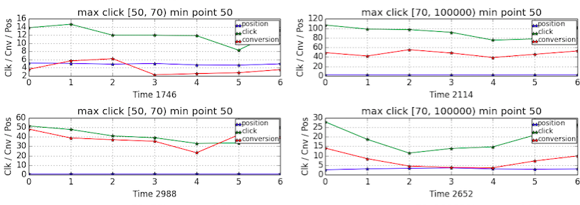
-
The following plot shows the availability of data in the space of keyword-campaign-time.
-
Collapse data by summing along the campaign dimension. The following figures shows the keywords-time matrices for different match types.
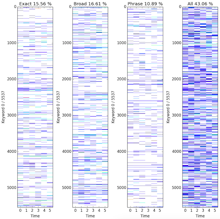
-
This is not too bad as half of the entries are missing.
Collaborative filtering
-
The first thing to do is to impute missing values by collaborative filtering.
-
The following table shows the statistics of the matrix I will be working with.
Item Value Missing entry 18916 All entry 33222 Missing at 56.94 % Keywords 5537 Time 6 -
The following matrix shows the parameter selection of collaborative filtering on
clickdata.Rank Lambda NumIter RMSE 2 0.010 5 4.77 2 0.010 10 4.73 2 0.010 15 4.71 2 0.050 5 4.84 2 0.050 10 4.74 2 0.050 15 4.74 2 0.100 5 4.97 2 0.100 10 4.80 2 0.100 15 4.75 3 0.010 5 3.72 3 0.010 10 3.74 3 0.010 15 3.67 3 0.050 5 3.91 3 0.050 10 3.70 3 0.050 15 3.72 3 0.100 5 4.05 3 0.100 10 3.75 3 0.100 15 3.71 4 0.010 5 2.48 4 0.010 10 2.45 4 0.010 15 2.45 4 0.050 5 2.69 4 0.050 10 2.50 4 0.050 15 2.45 4 0.100 5 2.64 4 0.100 10 2.55 4 0.100 15 2.49 -
I compute the rooted mean square error RMSE on training data and compared with mean imputation approach for
clickdata. The result is shown in the following table.Method RMSE CF 2.45 Mean imputation 20.58 -
The following matrix shows the parameter selection of collaborative filtering on
conversiondata.Rank Lambda NumIter RMSE 2 0.010 5 4.75 2 0.010 10 4.73 2 0.010 15 4.75 2 0.050 5 4.80 2 0.050 10 4.73 2 0.050 15 4.74 2 0.100 5 5.02 2 0.100 10 4.77 2 0.100 15 4.74 3 0.010 5 3.76 3 0.010 10 3.74 3 0.010 15 3.70 3 0.050 5 3.84 3 0.050 10 3.72 3 0.050 15 3.69 3 0.100 5 4.06 3 0.100 10 3.75 3 0.100 15 3.71 4 0.010 5 2.51 4 0.010 10 2.46 4 0.010 15 2.45 4 0.050 5 2.75 4 0.050 10 2.48 4 0.050 15 2.49 4 0.100 5 2.58 4 0.100 10 2.58 4 0.100 15 2.49 -
I compute the rooted mean square error RMSE on training data and compared with mean imputation approach for
conversiondata. The result is shown in the following table.Method RMSE CF 2.45 Mean imputation 20.58 -
The following figure shows the results of imputation on
conversiondata of 6 keywords. Each subplot shows theconversionnumber ofkeywordalong time. Vertical lines correspond to non-missing data.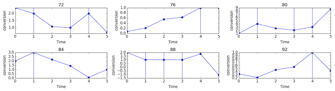
Learning and prediction
-
There are only information available for click and conversion data during the first 6 days and the task is to predict the click and conversion on 7 days.
-
It is somehow difficult to use the same regression approach as built for custom A.
-
For each keyword, the clicks/conversions in the first 6 day can be taken as a time series and the task can be translated into predict the click/conversion number on the 7 day.
-
Therefore, for each keyword, I build a autoregressive-moving-average ARMAR model trained on the time series of clicks and conversions.
-
Model tuning (parameter selection) is performed locally for each keyword.
-
The training rooted mean square error RMSE are shown in the following plot.
side note
- Learning can be improved by applying parameter selection on a training/validation/test partition other than current training/test partition.
- Parameter selection should be added to local random forest regression. For now, I only have parameter selection on collaborative filtering not for random forest regression.
- Paper on proper statistical test So you want to run an experiment …
- Parameter selection should be added to selecting rank parameter in autoregressive-moving-average ARMAR model.