Novelty detection and outlier detection with Scikit
Novelty detection and outlier detection with Scikit.
Table of content
Machine learning models
Novelty detection: one-class SVMs
One-class SVM is often used in novelty detection problem in which a clean labelled one class dataset is assume known apriori. The training is to separate all data points from origin with a maximized margin. Once the model is trained on the clean dataset, it is used to predict novelties which are the points located around the classification boundary/frontier. One good thing with one-class SVM is that the model is able to detect non-linear patterns using kernel function e.g., Gaussian RBF kernel.
Outlier detection: robust covariance estimation
Compared to one-class SVM, robust covariance estimation is designed for outlier detection problem in which we usually we have a mixture dataset with inliers and few outliers. The model estimate the variance of the dataset and detect the outliers when the actual variance of the data point is larger than the detected variance of the original dataset.
Empirical evaluations
In this section, I will test the performance of two algorithms described above in the context of outlier detection. In particular, robust covariance estimation is designed for outlier detection, one-class SVM designed for novelty detection is degraded into the same context.
Experiment settings
Let’s assume that data points are located in 2 dimensional space described by x and y coordinates. Inliers are generate from some Gaussian distributions with fixed means and standard derivations. Outliers are generated from a uniform distribution from the same space. In particular, I generate four different datasets. Each dataset consist of four 2D Gaussian distributions with \(\sigma=0.3\) and \(\mu\) from [(0,0),(0,0),(0,0),(0,0)] to [(4,4),(-4,-4),(-4,4),(4,-4)]. One-class SVMs and robust variance detection models are then applied to these four datasets.
Results
Classification errors of two models in four datasets are shown in the following table
| Dataset | One-class SVM | Variance detection |
|---|---|---|
| 1 | 6 | 6 |
| 2 | 26 | 6 |
| 3 | 40 | 54 |
| 4 | 46 | 98 |
I also plot the decision boundary of two models in the following figures.
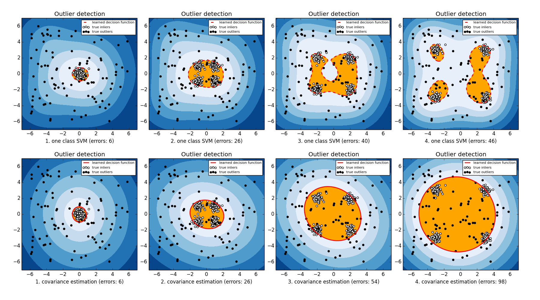
From the results, we can observe that when there exist clear cluster structures in the dataset one-class SVM is able to capture the cluster structured with Gaussian kernels. On the other hand, robust covariance estimation fails to capture the cluster structure and tries to estimate a covariance based on all data points from different clusters which lead to a drop of the performance when more cluster are presented.
Code
Python code that is used to generate the experiments is shown in the following code block.
1
2
3
4
5
6
7
8
9
10
11
12
13
14
15
16
17
18
19
20
21
22
23
24
25
26
27
28
29
30
31
32
33
34
35
36
37
38
39
40
41
42
43
44
45
46
47
48
49
50
51
52
53
54
55
56
57
58
59
60
61
62
63
64
65
66
67
68
69
70
71
72
73
74
75
76
'''
Outlier detection with one-class SVMs and robust covariance estimation.
One-class SVM is designed for novelty detection.
Robust covariance estimation is designed for outlier detection.
Code is modify from example in scikit-learn http://scikit-learn.org/stable/_downloads/plot_outlier_detection.py
Copyright @ Hongyu Su (hongyu.su@me.com)
'''
print (__doc__)
# scikit-learn package
from sklearn import svm
from sklearn.covariance import EllipticEnvelope
# numpy
import numpy as np
# plot
import matplotlib.pyplot as plt
import matplotlib.font_manager
from scipy import stats
n_samples=400
outliers_fraction=0.25
clusters_separation=[0,1,2,3]
# define classifier
classifiers = {'one class SVM': svm.OneClassSVM(nu=0.95*outliers_fraction+0.05,kernel='rbf',gamma=0.1),
'covariance estimation':EllipticEnvelope(contamination=0.1)}
xx, yy = np.meshgrid(np.linspace(-7, 7, 500), np.linspace(-7, 7, 500))
n_inliers = int((1. - outliers_fraction) * n_samples)
n_outliers = int(outliers_fraction * n_samples)
ground_truth = np.ones(n_samples, dtype=int)
ground_truth[-n_outliers:] = 0
# Fit the problem with varying cluster separation
plt.figure(figsize=(16,8))
for i, offset in enumerate(clusters_separation):
    np.random.seed(42)
    # generate inlier, gaussian
    x = 0.3 * np.random.randn(0.25 * n_inliers, 1) - offset
    y = 0.3 * np.random.randn(0.25 * n_inliers, 1) - offset
    X1 = np.r_[x,y].reshape((2,x.shape[0])).T
    x = 0.3 * np.random.randn(0.25 * n_inliers, 1) - offset
    y = 0.3 * np.random.randn(0.25 * n_inliers, 1) + offset
    X2 = np.r_[x,y].reshape((2,x.shape[0])).T
    x = 0.3 * np.random.randn(0.25 * n_inliers, 1) + offset
    y = 0.3 * np.random.randn(0.25 * n_inliers, 1) - offset
    X3 = np.r_[x,y].reshape((2,x.shape[0])).T
    x = 0.3 * np.random.randn(0.25 * n_inliers, 1) + offset
    y = 0.3 * np.random.randn(0.25 * n_inliers, 1) + offset
    X4 = np.r_[x,y].reshape((2,x.shape[0])).T
    X = np.r_[X1, X2, X3, X4]
    # generate outlier, uniform
    X = np.r_[X, np.random.uniform(low=-6, high=6, size=(n_outliers, 2))]
    # Fit the model with the One-Class SVM
    for j, (clf_name, clf) in enumerate(classifiers.items()):
        # fit the data and tag outliers
        clf.fit(X)
        y_pred = clf.decision_function(X).ravel()
        threshold = stats.scoreatpercentile(y_pred,100 * outliers_fraction)
        y_pred = y_pred > threshold
        n_errors = (y_pred != ground_truth).sum()
        # plot the levels lines and the points
        Z = clf.decision_function(np.c_[xx.ravel(), yy.ravel()])
        Z = Z.reshape(xx.shape)
        subplot = plt.subplot(2, 4, (j)*4+i+1)
        subplot.set_title("Outlier detection")
        subplot.contourf(xx, yy, Z, levels=np.linspace(Z.min(), threshold, 7),cmap=plt.cm.Blues_r)
        a = subplot.contour(xx, yy, Z, levels=[threshold],linewidths=2, colors='red')
        subplot.contourf(xx, yy, Z, levels=[threshold, Z.max()],colors='orange')
        b = subplot.scatter(X[:-n_outliers, 0], X[:-n_outliers, 1], c='white')
        c = subplot.scatter(X[-n_outliers:, 0], X[-n_outliers:, 1], c='black')
        subplot.axis('tight')
        subplot.legend(
            [a.collections[0], b, c],
            ['learned decision function', 'true inliers', 'true outliers'],
            prop=matplotlib.font_manager.FontProperties(size=8))
        subplot.set_xlabel("%d. %s (errors: %d)" % (i + 1, clf_name, n_errors))
        subplot.set_xlim((-7, 7))
        subplot.set_ylim((-7, 7))
    plt.subplots_adjust(0.04, 0.1, 0.96, 0.94, 0.1, 0.26)
plt.show()